Introduction
The Historic Volatility indicator is used mainly as an option evaluation
tool. It does not give trading signals like those given with other
technical indicators. What it does do is give the trader an idea of how
volatile the market has been for a previous period of time.
Changing the period of time the study observes allows the trader to fine
tune options prices. If a market has been extremely volatile for the
past 3 months, for example, then near term options should be more
expensive. If the market has been calm for an extended period of time,
longer term options should be reasonable.
Its use in futures is for observation, telling the trader if prices are
calming down or becoming more erratic.
Interpretation
The key to using historic volatility is determining the correct period
of time for each market. The market you are looking at may show a
history of volatility years ago, but may have been relatively calm the
last few months. Getting an idea of the markets behavior recently may be
of no use to the trader that is looking at distant options and vice
versa for the trader looking at near term options.
For the futures trader this tool is useful as a guide for order
placement. Seeing that market volatility is changing may indicate that
it is time to move stops closer or farther away. If the trader is
profitable with the trend and volatility is changing, it might be a time
to move stops closer to protect profits. If a trader is trading against
the trend, they might want to move stops further away to avoid getting
bumped out prematurely.
Options traders could use this study to help them purchase profitable
options. The basic idea is to buy options when volatility is decreasing
to take advantage of a change in that volatility. Any rise in volatility
will translate to an increase in option values. Look at options
strategies that take advantage of low volatility, such as straddles or
ratio spreads. When volatility is high, selling options would be better
because any decrease in volatility will translate to a loss of option
value. Option strategies that take advantage of a decrease in volatility
are strangles and regular short option positions.
Obviously, historic volatility is only one component of option pricing.
Any changes in the underlying futures market could negate the changes in
option prices due to volatility. For example, if you were to buy a low
volatility Put option and prices go higher, that option will lose value
but not as quickly as a higher volatility option.
For the futures trader the basic concept is to expect market changes
during periods of increased volatility. George Soros, the trading
legend, said "Short term volatility is greatest at a turn around and
diminishes as a trend becomes established."
This indicator is commonly viewed as very mean regressive. What this
term means is that the historic volatility indicator tends to return to
the opposite end of the spectrum and therefore return to an average. If
volatility is great it will eventually cool off and return to that
place. If volatility is low it will not stay quiet forever. What this
means to traders is that a market that is erratic will sooner or later
calm down and a market that is quiet will eventually get loud again.
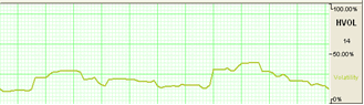
Example of Historical Velocity in the Indicator Window:
Calculation
Parameters:
Period (20) - the number of bars, or period, used to calculate the
study. You may alter this to use any number greater than 1 for the
close. The indicator displays simple percentage values.
Formula:
The calculation for the historical volatility is rather involved. The
number of periods per year vary depending on the type of price chart
used for the study. The following table lists the number of periods for
each type of chart:
| Chart Type |
Trading
Periods per Year |
| Perpetual |
262 |
| Daily |
262 |
| Weekly |
52 |
| Monthly |
12 |
| Variable |
Based on chart
period (see below) |
| Tick |
Not available
for this study |
When using variable charts, you must
first calculate the number of trading periods per year. To do this, you
must determine the trading time of the selected commodity. The formula
is as follows:
TP = (Tt / Pn) * 262
TP: The total number of trading periods per year.
Tt: The total trading time in a day.
Pn: The length of the period.
262: The number of weekdays per year. Example: The S&P 500 trades from 8:30 a.m. to 3:15 p.m. That is a
total trading time of 6 hours and 45 minutes. On a variable chart using
5 minute bars, the number of periods for the day is 81 as demonstrated:
6 hours @ 60 minutes = 360 minutes
45 minutes +45 minutes
Total minutes of trading = 405 minutes
405 / 5 minute bars = 81 trading periods per day Now that you have calculated the trading periods per day, you now must
calculate the number of periods for the year. Since historical
volatility considers every weekday of the year when calculating total
periods for the year, the multiplier is 262:
TP = (405)/5) * 262
TP = 81* 262
TP = 21,222
Note: This formula applies only to historical volatility on a
variable chart. It does not apply to other chart types.
Now that you have the total number of periods per year, continue with
the calculation of the historical volatility.
Next calculate the logarithm of the price change for each price in the
specified time span of n periods. The formula is:
LOGSi = LOG(Pi / Pi-1)
LOG: The logarithm function.
Pi: The current price.
Pi-1: The previous price. Now that you have the logarithms of the price changes, calculate the
total logarithms for the time span you are reviewing. To calculate the
total of the logarithms, use the following formula:
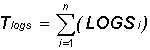
Tlogs: The total of the logarithm price ratio for the time span.
S: Indicates to sum all n logarithms.
LOGSi: The logarithm of the price change for period i.
N: The number of periods for the specified time span.
The next step is to calculate the average of the logs by dividing the
total logarithm by the number of periods as shown below:
ALOGS = Tlogs / n
ALOGS: The average of the logarithms.
Tlogs: The total of the logarithm for the time span.
N: The number of periods for the specified time span. The last calculation is to sum the squares of the difference between the
individual logarithms for each period and the average logarithm. This is
accomplished in the following formula:
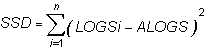
SSD: The sum of the squared differences.
S: Indicates to total the squares of all n differences.
LOGSi: The logarithm of the price change for period i.
ALOGS: The average of the logarithms.
Now that the elements of the final formula are complete, the following
formula calculates the historical volatility for a given period over a
specified time span.
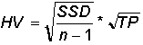
SSD: The sum of the squared differences.
n: The number of periods for the specified time span.
TP: The total number of trading periods for the year. Due to the complexity of the formula, it is preferable to use a
scientific calculator when attempting to manually calculate the
historical volatility of a futures instrument.
Customizing
To change the settings of this indicator, open the Program Options
screen by clicking the "Program Options" button located on the main
Toolbar.
See the Program Options section for more details on changing the
settings.
Back
To Top |